Lab02: Distances and the Border Zone

Ecosystem Science and Sustanability 523c

Author

Billy Johnson

Load in the libraries

# spatial data science
library(tidyverse)
library(sf)
library(units)

# Data
library(USA.state.boundaries)
library(rnaturalearth)

# Visualization
library(gghighlight)
library(ggrepel)
library(knitr)
library(flextable)
library(leaflet)
library(ggthemes)

# Other
library(readr)

Question 1

1.1 Define a projection

Use North America Equidistant Conic

eqdc <- '+proj=eqdc +lat_0=40 +lon_0=-96 +lat_1=20 +lat_2=60 +x_0=0 +y_0=0 +datum=NAD83 +units=m +no_defs'

1.2 Get USA state boudaries

remotes::install_github("ropensci/USAboundaries")

Using GitHub PAT from the git credential store.

Skipping install of 'USAboundaries' from a github remote, the SHA1 (0f56f492) has not changed since last install.
  Use `force = TRUE` to force installation

remotes::install_github("ropensci/USAboundariesData")

Using GitHub PAT from the git credential store.

Skipping install of 'USAboundariesData' from a github remote, the SHA1 (064cdbcb) has not changed since last install.
  Use `force = TRUE` to force installation

# Once installed
USA_states_raw <- USAboundaries::us_states(resolution = "low")

1.3 Get country boundaries for Mexico, the US and Canada

remotes::install_github("ropenscilabs/rnaturalearthdata")

Using GitHub PAT from the git credential store.

Skipping install of 'rnaturalearthdata' from a github remote, the SHA1 (ff4d891f) has not changed since last install.
  Use `force = TRUE` to force installation

countries <- rnaturalearth::countries110 %>% 
  st_as_sf() %>% 
  filter(countries110$ADMIN %in% c("United States of America", "Canada", "Mexico")) %>% 
  st_transform(crs = eqdc)

1.4 Get city locations from the csv file

city_locations <- read_csv("Lab2/simplemaps_uscities_basicv1/uscities.csv")

Rows: 31254 Columns: 17
── Column specification ────────────────────────────────────────────────────────
Delimiter: ","
chr (9): city, city_ascii, state_id, state_name, county_fips, county_name, s...
dbl (6): lat, lng, population, density, ranking, id
lgl (2): military, incorporated

ℹ Use `spec()` to retrieve the full column specification for this data.
ℹ Specify the column types or set `show_col_types = FALSE` to quiet this message.

city_locations_clean <- city_locations %>% 
  filter(!state_id %in% c("AK", "HI", "PR"))

# Convert to spatial
city_location_sp <- st_as_sf(city_locations_clean,
                             coords = c("lng", "lat"),
                             crs = 4326) %>% 
  select(city, population, state_name) %>% 
  st_transform(crs = eqdc)


#st_filter(city_location_sp,
#          filter(city_location_sp, city == "Fort Collins"),
#          .predicate = st_is_within_distance, 1000)

Question 2

2.1 Distance to USA border (coastline or national) (km)

# Convert USA state boundaries to a MULTILINESTRING
USA_border <- USA_states_raw %>% 
  filter(!state_abbr %in% c("AK", "HI", "PR")) %>% 
  st_union() %>% 
  st_cast("MULTILINESTRING") %>% 
  st_transform(crs = eqdc)

# CREATE DISTANCE COLUMN
city_location_sp$dist_us_border_km <- st_distance(city_location_sp, USA_border) %>% 
  set_units("km") %>% 
  drop_units()

# Create flextable
top5_us_border <- city_location_sp %>% 
  slice_max(order_by = dist_us_border_km, n = 5) %>% 
  select(city, state_name, dist_us_border_km) %>% 
  flextable() %>% 
  set_caption("Top 5 US cities with the greatest distance to the US border")

top5_us_border


city	state_name	dist_us_border_km	geometry
Ludell	Kansas	1,012.508	[[XY]]
Dresden	Kansas	1,012.398	[[XY]]
Herndon	Kansas	1,007.763	[[XY]]
Hill City	Kansas	1,005.140	[[XY]]
Atwood	Kansas	1,004.734	[[XY]]

2.2 Distance to state borders

# Create US state borders
state_borders <- USA_states_raw %>% 
  filter(!state_abbr %in% c("AK", "HI", "PR")) %>% 
  st_combine() %>% 
  st_cast("MULTILINESTRING") %>% 
  st_transform(crs = eqdc) 

# Calculate the distances to state border
city_location_sp$dist_state_border_km <- st_distance(city_location_sp, state_borders) %>% 
  set_units("km") %>% 
  drop_units()

# Create table
top5_state_border <- city_location_sp %>% 
  slice_max(order_by = dist_state_border_km, n = 5) %>% 
  select(city, state_name, dist_state_border_km) %>% 
  flextable() %>% 
  set_caption("Top 5 US cities with the greatest distance to the state border")

top5_state_border


city	state_name	dist_state_border_km	geometry
Briggs	Texas	309.4150	[[XY]]
Lampasas	Texas	308.9216	[[XY]]
Kempner	Texas	302.5868	[[XY]]
Bertram	Texas	302.5776	[[XY]]
Harker Heights	Texas	298.8138	[[XY]]

2.3 Distance to Mexico

mexico <- countries %>% 
  filter(ADMIN == "Mexico") %>% 
  st_union() %>% 
  st_cast("MULTILINESTRING") %>% 
  st_transform(crs = eqdc)

city_location_sp$dist_mexico_km <- st_distance(city_location_sp, mexico) %>% 
  set_units("km") %>% 
  drop_units()

top5_mexico <- city_location_sp %>% 
  slice_max(order_by = dist_mexico_km, n = 5) %>% 
  select(city, state_name, dist_mexico_km) %>% 
  flextable() %>% 
  set_caption("Top 5 US cities longest distance to Mexico border")

top5_mexico


city	state_name	dist_mexico_km	geometry
Grand Isle	Maine	3,282.825	[[XY]]
Caribou	Maine	3,250.330	[[XY]]
Presque Isle	Maine	3,234.570	[[XY]]
Oakfield	Maine	3,175.577	[[XY]]
Island Falls	Maine	3,162.285	[[XY]]

2.4 Distance to Canada (km)

canada <- countries %>% 
  filter(ADMIN == "Canada") %>% 
  st_union() %>% 
  st_cast("MULTILINESTRING") %>% 
  st_transform(crs = eqdc)

city_location_sp$dist_canada_km <- st_distance(city_location_sp, canada) %>% 
  set_units("km") %>% 
  drop_units()

top5_canada <- city_location_sp %>% 
  slice_max(order_by = dist_canada_km, n = 5) %>% 
  select(city, state_name, dist_canada_km) %>% 
  flextable() %>% 
  set_caption("Top 5 US cities with the longest distance to the Canadian border")

top5_canada


city	state_name	dist_canada_km	geometry
Guadalupe Guerra	Texas	2,206.455	[[XY]]
Sandoval	Texas	2,205.641	[[XY]]
Fronton	Texas	2,204.794	[[XY]]
Fronton Ranchettes	Texas	2,202.118	[[XY]]
Evergreen	Texas	2,202.020	[[XY]]

Question 3

Visualization of distance data ### 3.1 Data

# Show the 3 continents, CONUS outline, state boundaries, and 10 largest USA cities (population) on a single map

top10_cities <- city_location_sp %>% 
  arrange(desc(population)) %>% 
  slice(1:10)

# Plot
ggplot()+
  geom_sf(data = countries, fill = "grey", color = "white", lty = "solid", size = 0.3)+
  geom_sf(data = USA_border, fill = NA, color = "black", lty = "dashed", size = 0.3)+
  geom_sf(data = state_borders, fill = NA, color = "black", lty = "solid", size = 0.05)+
  geom_sf(data = top10_cities, color = "red")+
  ggrepel::geom_label_repel(data = top10_cities, aes(label = city, geometry = geometry),
                            stat = "sf_coordinates",
                            size = 3)+
  theme_map()+
  labs(title = "Map of US top 10 most populated cities")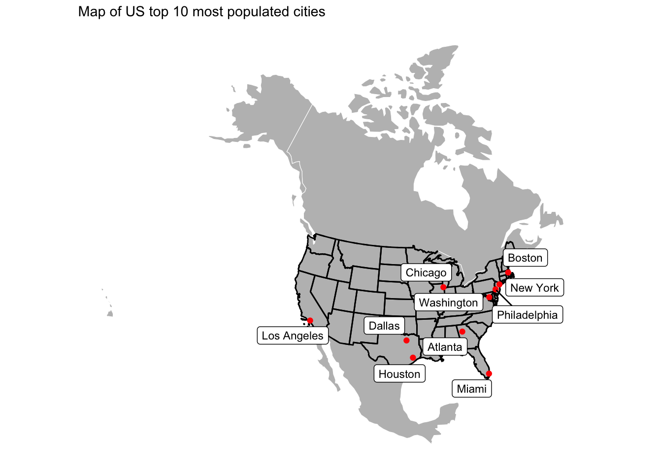

3.2 City Distance from the border

top5_city_distance <- city_location_sp %>% 
  arrange(desc(dist_us_border_km)) %>%
  slice(1:5) %>% 
  mutate(city_label = paste0(city, ",", state_name))


ggplot()+
  geom_sf(data = city_location_sp, aes(color = dist_us_border_km))+
  scale_color_viridis_c(option = "plasma")+
  labs(color = "Distance to US Border (km)")+
  ggrepel::geom_label_repel(data = top5_city_distance, aes(label = city_label, geometry = geometry),
                            stat = "sf_coordinates",
                            size = 3)+
  theme_map()+
  labs(title = "Cities in the US and the distance to the U.S. Border")

3.3 City Distance from Nearest state

top5_city_distance_state <- city_location_sp %>% 
  arrange(desc(dist_state_border_km)) %>%
  slice(1:5) %>% 
  mutate(city_label = paste0(city, ",", state_name))


ggplot()+
  geom_sf(data = city_location_sp, aes(color = dist_state_border_km))+
  scale_color_viridis_c(option = "plasma")+
  labs(color = "Distance to State Border (km)")+
  ggrepel::geom_label_repel(data = top5_city_distance_state, aes(label = city_label, geometry = geometry),
                            stat = "sf_coordinates",
                            size = 3)+
  theme_map()+
  labs(title = "City Distance to State Boundary")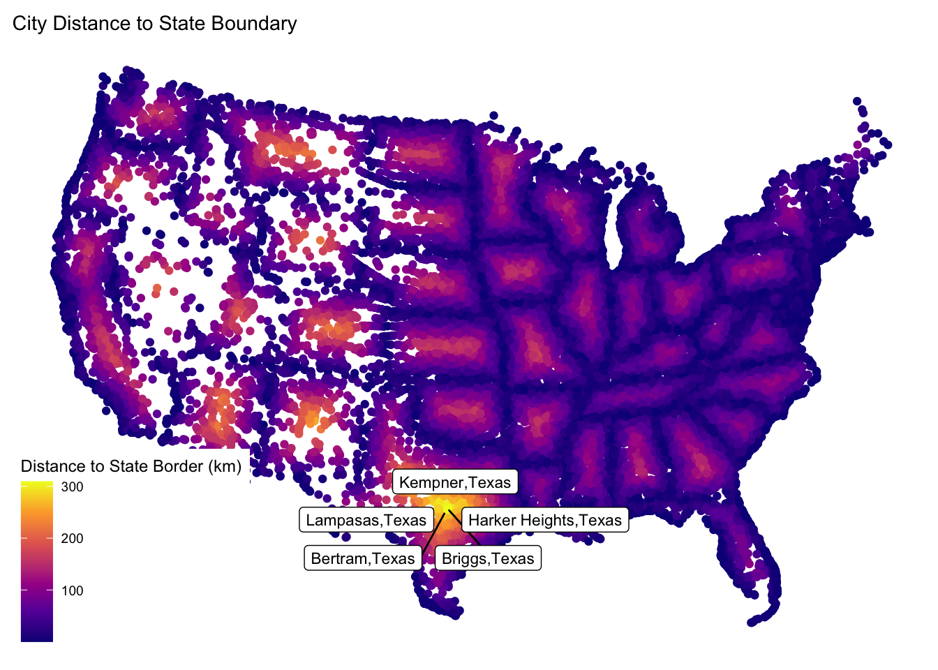

3.4 Equidistance boundary from Mexico and Canada

city_location_sp <- city_location_sp %>% 
  mutate(absolute_distance = abs(dist_mexico_km - dist_canada_km))

equal_distance_cities <- city_location_sp %>% 
  filter(absolute_distance <= 100)

Warning: Using one column matrices in `filter()` was deprecated in dplyr 1.1.0.
ℹ Please use one dimensional logical vectors instead.

top5_pop_cities_near_border <- equal_distance_cities %>% 
  arrange(desc(population)) %>% 
  slice_head(n =5)

ggplot()+
  geom_sf(data = city_location_sp, aes(color = absolute_distance))+
  gghighlight(absolute_distance <= 100, use_direct_label = FALSE)+
  ggrepel::geom_label_repel(data = top5_pop_cities_near_border,
                            aes(label = paste0(city, "," , state_name), geometry = geometry),
                            stat = "sf_coordinates",
                            size = 3)+
  scale_color_viridis_c(option = "inferno", name = "Distance Difference (km)")+
  theme_map()+
  labs(title = "Most Populous City in Each State Farthest Away from the U.S. Border")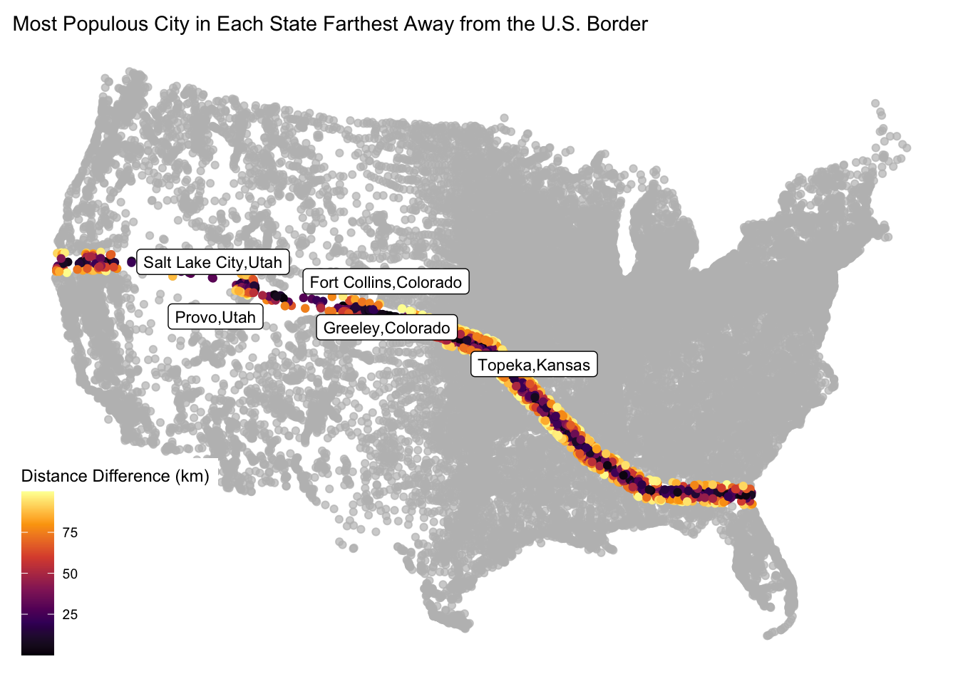

Question 4

Real World Application

4.1 Quantifing Border Zone

# Filter for cities in 100 mi or 160 km of border
border_zone_cities <- city_location_sp %>% 
  filter(dist_us_border_km <= 160) 

border_zone_populations <- border_zone_cities %>% 
  summarize(total_population = sum(population, na.rm = TRUE))

total_US_pop <- sum(city_location_sp$population)

percentage_pop <- border_zone_populations$total_population / total_US_pop * 100

summary_table <- data.frame(
  "Number of Cities in 100 Miles Zone" = nrow(border_zone_cities),
  "Total Population in Border Zone" = border_zone_populations$total_population,
  "Percentage of Total U.S. Population" = percentage_pop
)

summary_table

  Number.of.Cities.in.100.Miles.Zone Total.Population.in.Border.Zone
1                              13160                       256086824
  Percentage.of.Total.U.S..Population
1                            64.63109

flextable(summary_table, )

Number.of.Cities.in.100.Miles.Zone	Total.Population.in.Border.Zone	Percentage.of.Total.U.S..Population
13,160	256,086,824	64.63109

4.2 Mapping Border Zone

top10_border_zone <- border_zone_cities %>% 
  arrange(desc(population)) %>% 
  slice_head(n = 10)

ggplot()+
  geom_sf(data = city_location_sp, aes(color = dist_us_border_km))+
  gghighlight(dist_us_border_km <= 160, use_direct_label = FALSE)+
  scale_color_gradient(low = "orange", high = "darkred")+
  ggrepel::geom_label_repel(data = top10_border_zone,
                            aes(label = paste0(city, ",", state_name), geometry = geometry),
                            stat = "sf_coordinates",
                            size = 3)+
  theme_map()+
  labs(title = "10 most Populous Cities in U.S. within 100 Miles of the U.S. Border")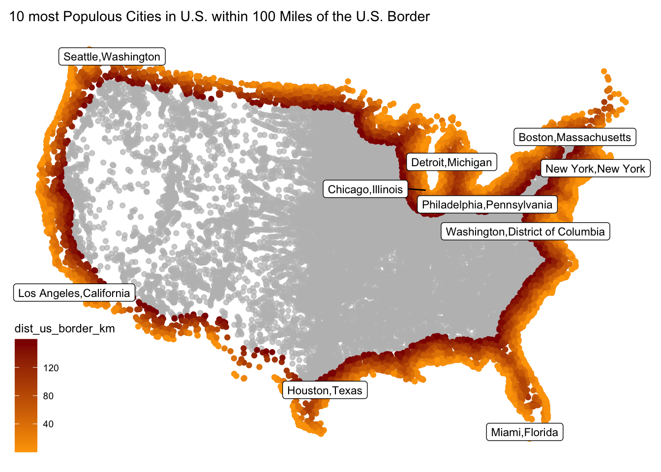

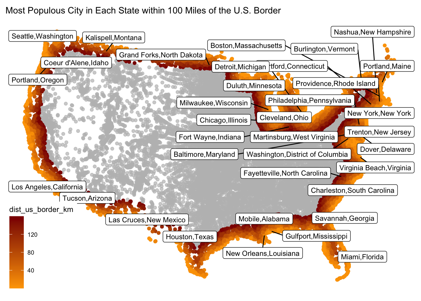
4.3 Instead of labeling the 10 most populous cities label the most populous cities in each state within the Danger Zone.

most_pop_cities_state <- border_zone_cities %>%
  filter(dist_us_border_km <= 160) %>% 
  group_by(state_name) %>% 
  slice_max(population, n =1) %>% 
  ungroup()

ggplot()+
  geom_sf(data = city_location_sp, aes(color = dist_us_border_km))+
  gghighlight(dist_us_border_km <= 160, use_direct_label = FALSE)+
  scale_color_gradient(low = "orange", high = "darkred")+
  ggrepel::geom_label_repel(data = most_pop_cities_state,
                            aes(label = paste0(city, ",", state_name), geometry = geometry),
                            stat = "sf_coordinates",
                            size = 3,
                            max.overlaps = 30)+
  theme_map()+
  labs(title = "Most Populous City in Each State within 100 Miles of the U.S. Border")