library(tidyverse)
library(sf)
library(rmapshaper)
library(units)
library(knitr)
library(kableExtra)
library(gghighlight)
library(leaflet)
library(leafem)Lab 03
National Dam Inventory
Question 1
Step 1.1
AOI <- remotes::install_github("mikejohnson51/AOI")Using GitHub PAT from the git credential store.Skipping install of 'AOI' from a github remote, the SHA1 (f821d499) has not changed since last install.
Use `force = TRUE` to force installationUS_counties <- AOI::aoi_get(state = "conus", county = "all")
US_counties_sf <- US_counties %>%
st_transform(crs = "EPSG:5070")Step 1.2
counties_centroid <- US_counties_sf %>%
  st_centroid()
Warning: st_centroid assumes attributes are constant over geometriescounty_points <- st_union(counties_centroid)Step 1.3
# Voroni
voroni_tessellation <- st_voronoi(county_points)%>%
  st_as_sf() %>%
  mutate(id = 1:n()) %>%
  st_cast()
Warning in st_cast.sf(.): repeating attributes for all sub-geometries for which
they may not be constant# Triangulated
triangulated_tessellation <- st_triangulate(county_points)%>%
st_as_sf() %>%
mutate(id = 1:n()) %>%
st_cast()Warning in st_cast.sf(.): repeating attributes for all sub-geometries for which
they may not be constant# Gridded Coverage
gridded_coverage <- st_make_grid(county_points, n = 70)%>%
st_as_sf() %>%
mutate(id = 1:n()) %>%
st_cast()
# Hexagonal coverage
hexegonal_coverage <- st_make_grid(county_points, square = FALSE, n = 70) %>%
st_as_sf() %>%
mutate(id = 1:n()) %>%
st_cast()Step 1.4
conus_boundary <- st_union(US_counties_sf)

# Voroni
USA_voroni <- st_intersection(voroni_tessellation, conus_boundary)
Warning: attribute variables are assumed to be spatially constant throughout
all geometries# Triangulate
USA_triangulate <- st_intersection(triangulated_tessellation, conus_boundary)Warning: attribute variables are assumed to be spatially constant throughout
all geometries# Gridded
USA_gridded <- st_intersection(gridded_coverage, conus_boundary)Warning: attribute variables are assumed to be spatially constant throughout
all geometries# Hexegonal
USA_hexegonal <- st_intersection(hexegonal_coverage, conus_boundary)Warning: attribute variables are assumed to be spatially constant throughout
all geometriesStep 1.5
# Simplify unioned border
simple_USA_boundary <- ms_simplify(conus_boundary, keep = 0.05)
Number of points
mapview::npts(conus_boundary)[1] 11292mapview::npts(simple_USA_boundary)[1] 577Doing the simplification step I was able to remove 10,715 points. Some consequences of doing this computationally may lead to removal of important features.
Crop triangulated tessellations
USA_triangulate_crop <- st_intersection(USA_triangulate, simple_USA_boundary)Warning: attribute variables are assumed to be spatially constant throughout
all geometriestriangulate_tessellation_crop <- st_intersection(triangulated_tessellation, simple_USA_boundary)Warning: attribute variables are assumed to be spatially constant throughout
all geometriesStep 1.6
# Write function to plot tessellations
tessellation_plot_funct <- function(arg1, arg2){
  ggplot(data = arg1)+
    geom_sf(fill = "white", color = "navy", size = 0.2)+
    theme_void()+
    labs(
      title = arg2,
      caption = paste("Number of features in arg 1 = ", nrow(arg1)))
}
Step 1.7
Voroni Tessellation
tessellation_plot_funct(USA_voroni, "Voroni Tessellation")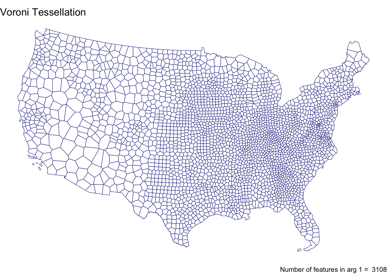
Triangulate Tessellation
tessellation_plot_funct(USA_triangulate_crop, "Triangulate Tessellation")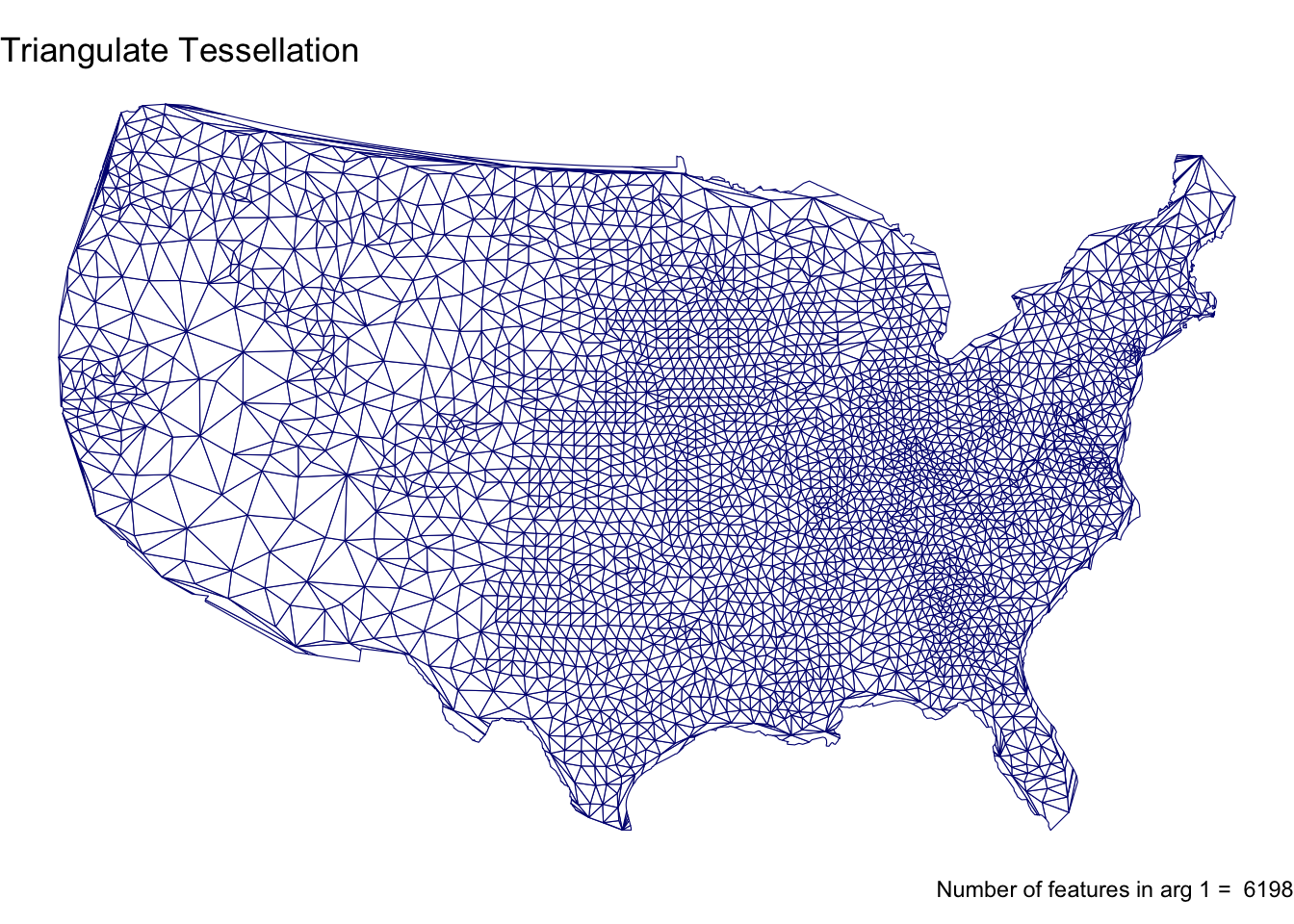
Square Grid Coverage
tessellation_plot_funct(USA_gridded, "Square Grid Coverage")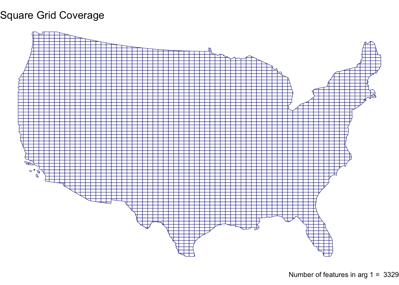
Hexagonal Grid Coverage
tessellation_plot_funct(USA_hexegonal, "Hexagonal Grid Coverage")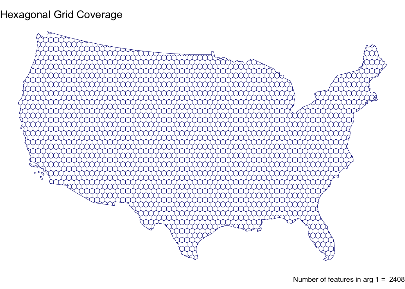
Original County Data
tessellation_plot_funct(US_counties_sf, "Original County Data")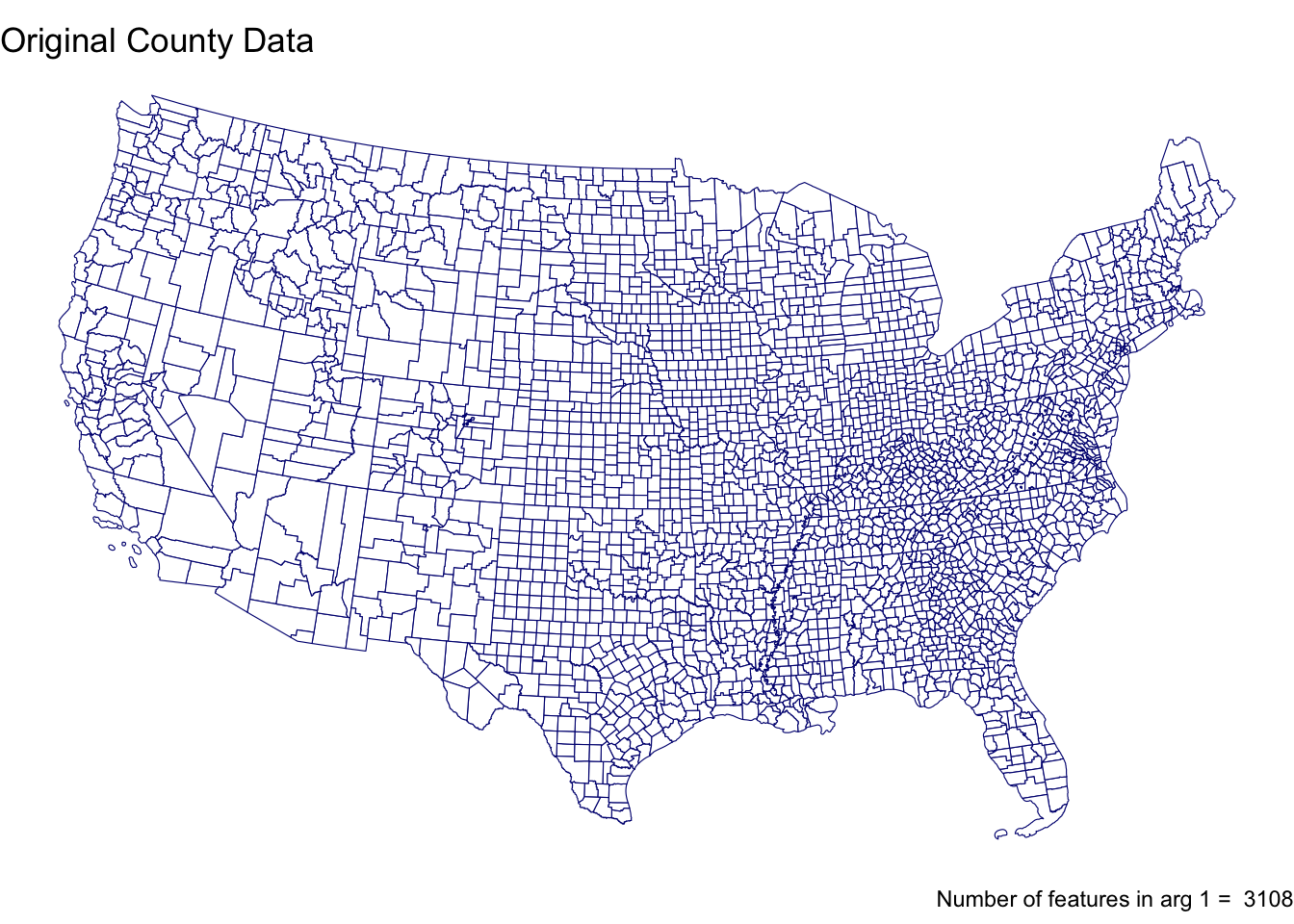
Question 2
Step 2.1
Create function for turning SF object and Character string to return data.frame
tessellated_surfaces_funct <- function(arg1, arg2) {
  areas_km2 <- st_area(arg1) %>%
    set_units(km^2) %>%
    drop_units()

  summary_df <- data.frame(
    description = arg2,
    num_features = nrow(arg1),
    mean_area_km2 = mean(areas_km2),
    sd_area_km2 = sd(areas_km2),
    total_area_km2 = sum(areas_km2)
  )

  return(summary_df)
}
Step 2.2
Summarize each of the tessellations and the original counties
Voroni Tessellation Surface Summary
V_sum <- tessellated_surfaces_funct(USA_voroni, "Voroni Tessellated Surfaces")

V_sum| description | num_features | mean_area_km2 | sd_area_km2 | total_area_km2 |
|---|---|---|---|---|
| Voroni Tessellated Surfaces | 3108 | 2605.05 | 2918.74 | 8096496 |
Triangulated Tessellation Surface Summary
T_sum <- tessellated_surfaces_funct(USA_triangulate_crop, "Triangulated Tessellation Surface Summary")

T_sum| description | num_features | mean_area_km2 | sd_area_km2 | total_area_km2 |
|---|---|---|---|---|
| Triangulated Tessellation Surface Summary | 6198 | 1289.78 | 1597.416 | 7994054 |
Square Grid Surface Summary
SG_sum <- tessellated_surfaces_funct(USA_gridded, "Square Grid Surface Summary")

SG_sum| description | num_features | mean_area_km2 | sd_area_km2 | total_area_km2 |
|---|---|---|---|---|
| Square Grid Surface Summary | 3329 | 2423.591 | 504.1926 | 8068134 |
Hexagonal Grid Surface Summary
H_sum <- tessellated_surfaces_funct(USA_hexegonal, "Hexagonal Grid Surface Summary")

H_sum| description | num_features | mean_area_km2 | sd_area_km2 | total_area_km2 |
|---|---|---|---|---|
| Hexagonal Grid Surface Summary | 2408 | 3359.835 | 748.5251 | 8090484 |
Original County Surface Summary
O_sum <- tessellated_surfaces_funct(US_counties_sf, "Original County Surface Summary")

O_sum| description | num_features | mean_area_km2 | sd_area_km2 | total_area_km2 |
|---|---|---|---|---|
| Original County Surface Summary | 3108 | 2605.05 | 3443.712 | 8096496 |
Step 2.3
tesselation_summaries <- bind_rows(V_sum, T_sum, SG_sum, H_sum, O_sum)

tesselation_summaries| description | num_features | mean_area_km2 | sd_area_km2 | total_area_km2 |
|---|---|---|---|---|
| Voroni Tessellated Surfaces | 3108 | 2605.050 | 2918.7397 | 8096496 |
| Triangulated Tessellation Surface Summary | 6198 | 1289.780 | 1597.4161 | 7994054 |
| Square Grid Surface Summary | 3329 | 2423.591 | 504.1926 | 8068134 |
| Hexagonal Grid Surface Summary | 2408 | 3359.835 | 748.5251 | 8090484 |
| Original County Surface Summary | 3108 | 2605.050 | 3443.7121 | 8096496 |
Step 2.4
Print data frame as a nice table
tesselation_summaries %>%
kable(digits = 2, caption = "Summary of differnt Tessellation Methods for the United States Counties", format = "html")| description | num_features | mean_area_km2 | sd_area_km2 | total_area_km2 |
|---|---|---|---|---|
| Voroni Tessellated Surfaces | 3108 | 2605.05 | 2918.74 | 8096496 |
| Triangulated Tessellation Surface Summary | 6198 | 1289.78 | 1597.42 | 7994054 |
| Square Grid Surface Summary | 3329 | 2423.59 | 504.19 | 8068134 |
| Hexagonal Grid Surface Summary | 2408 | 3359.84 | 748.53 | 8090484 |
| Original County Surface Summary | 3108 | 2605.05 | 3443.71 | 8096496 |
Step 2.5
Voroni polygons are variable in shape and size. Because these types of tessellations are adaptive to data they are very sensitive to changes. We also see that in the triangulated tessellation because these are variable in shape and size and are dependent on the data. This differed in the other methods square and hexagonal. These are fixed shapes and sizes. They just help interpret the data in a country balanced view.
Question 3
Step 3.1
# Load in the Dam invintory data
dam_data_raw <- read_csv("NID2019_U.csv")
Rows: 91457 Columns: 69
── Column specification ────────────────────────────────────────────────────────
Delimiter: ","
chr (44): DAM_NAME, OTHER_DAM_NAME, DAM_FORMER_NAME, NIDID, SECTION, COUNTY,...
dbl (24): RECORDID, STATEID, LONGITUDE, LATITUDE, DISTANCE, YEAR_COMPLETED, ...
lgl (1): URL_ADDRESS
ℹ Use `spec()` to retrieve the full column specification for this data.
ℹ Specify the column types or set `show_col_types = FALSE` to quiet this message.usa <- AOI::aoi_get(state = "conus") %>%
st_union() %>%
st_transform(5070)
dams <- dam_data_raw %>%
filter(!is.na(LATITUDE)) %>%
st_as_sf(coords = c("LONGITUDE", "LATITUDE"), crs = 4236) %>%
st_transform(5070) %>%
st_filter(usa)Step 3.2
Create points in polygon function
points_in_polygon <- function(points, polygon, var){
  st_join(polygon, points) %>%
    st_drop_geometry() %>%
    count(get(var)) %>%
    setNames(c(var, "n")) %>%
    left_join(polygon, by = var) %>% st_as_sf()
}
Step 3.3
Voroni Tessellation
V_dam <- points_in_polygon(dams, USA_voroni, "id")Triangulated Tessellation
T_dam <- points_in_polygon(dams, USA_triangulate_crop, "id")Square Grid Coverage
S_dam <- points_in_polygon(dams, USA_gridded, "id")Hexagonal Grid Coverage
H_dam <- points_in_polygon(dams, USA_hexegonal, "id")Original County
# O_dam <- points_in_polygon(dams, US_counties_sf, "id")Step 3.4
Create function for plotting dams
# Dam plotting function
dam_plot_funct <- function(arg1, arg2){
  ggplot(data = arg1)+
    geom_sf(aes(fill = n), color = NA)+
    scale_fill_viridis_c(option = "D", name = "Number of Dams")+
    theme_void()+
    labs(
      title = arg2,
      caption = paste("Total Number of Dams = ", sum(arg1$n, na.rm = TRUE)))
}
Step 3.5
Voroni Dam Plot
dam_plot_funct(V_dam, "Voroni Tesselation Dam Map")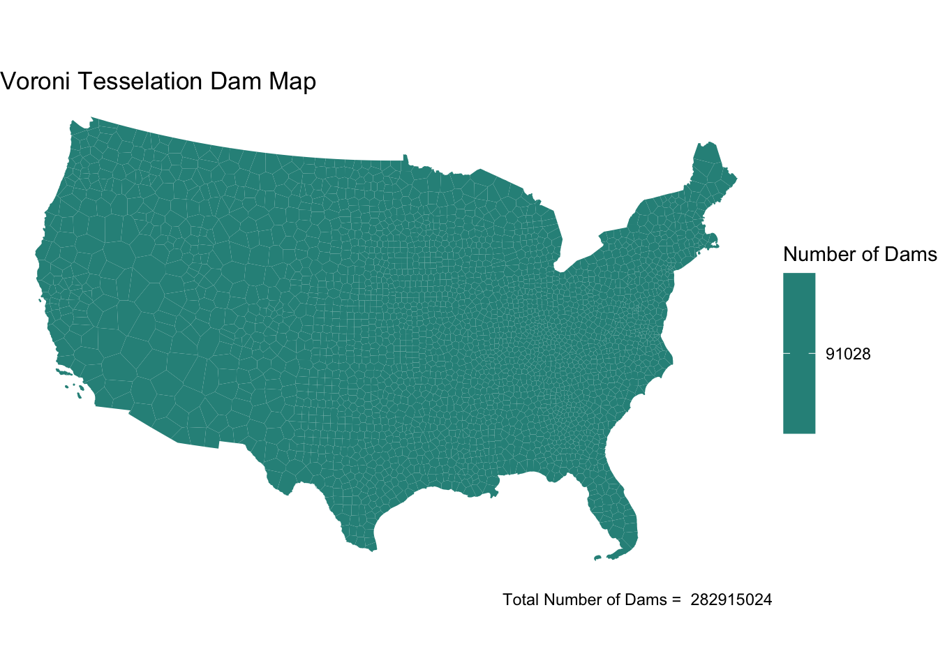
Triangulated Dam Plot
dam_plot_funct(T_dam, "Triangulated Tesselation Dam Map")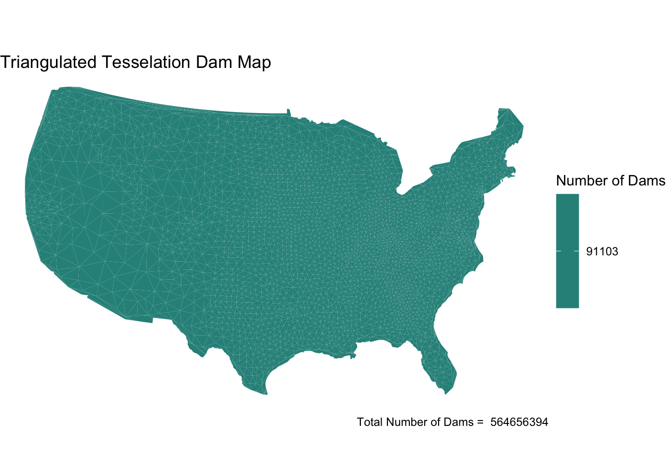
Square Gridded Dam Plot
dam_plot_funct(S_dam, "Squared Gridded Coverage Dam Map")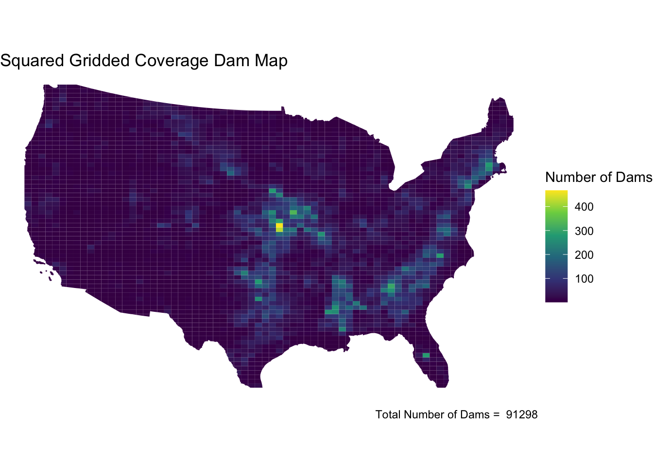
Hexagonal Grid Dam Plot
dam_plot_funct(H_dam, "Hexagonal Grid Coverage Dam Map")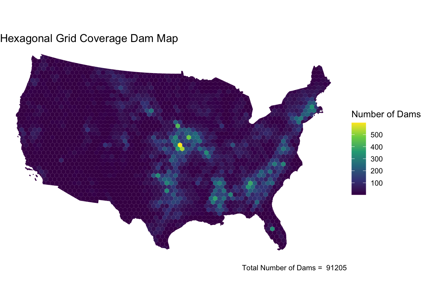
Step 3.6
the influence of the tessellated surfaces was shocking to me. The two coverage tactics showed results while the vorni and triangulated methods seemed to have to big of tiles to pull information. To move on I will be useing the hexagonal tessellation. This view seemed to be balanced and not to big and was able to also not create clustering effects.
Question 4
Step 4.1
Choose 4 dam purposes C - Flood Control I - Irrigation S - Water Supply F - Fish and Wildlife
flood_dams <- dams %>% filter(grepl("C", PURPOSES))

Irrigation_dams <- dams %>% filter(grepl("I", PURPOSES))

Supply_dams <- dams %>% filter(grepl("S", PURPOSES))

Fish_dams <- dams %>% filter(grepl("F", PURPOSES))
Run the points in polygons with hexagonal grid coverage tessellation
# flood
Hex_flood <- points_in_polygon(flood_dams, USA_hexegonal, "id")
# Irrigation
Hex_irrigation <- points_in_polygon(Irrigation_dams, USA_hexegonal, "id")
# Water Supply
Hex_supply <- points_in_polygon(Supply_dams, USA_hexegonal, "id")
# Fish
Hex_fish <-
points_in_polygon(Fish_dams, USA_hexegonal, "id")
Step 4.2
plot
threshold <- mean(Hex_flood$n, na.rm = TRUE) + sd(Hex_flood$n, na.rm = TRUE)Flood Control Dams
dam_plot_funct(Hex_flood, "Flood Control Dams") +
  gghighlight(n > threshold)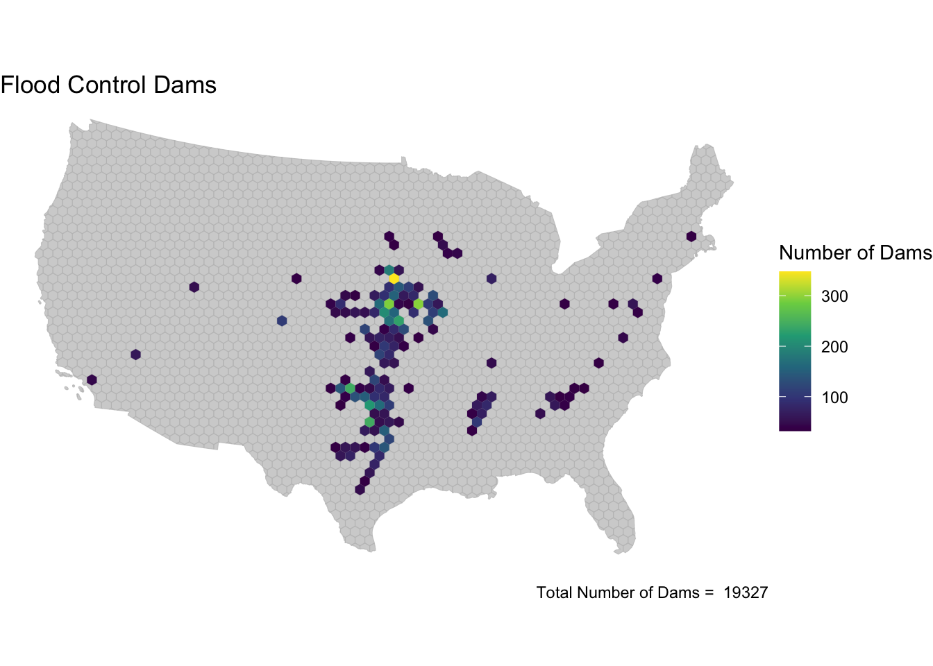
Irrigation Dams
dam_plot_funct(Hex_irrigation, "Irrigation Dams")+
  gghighlight(n > threshold)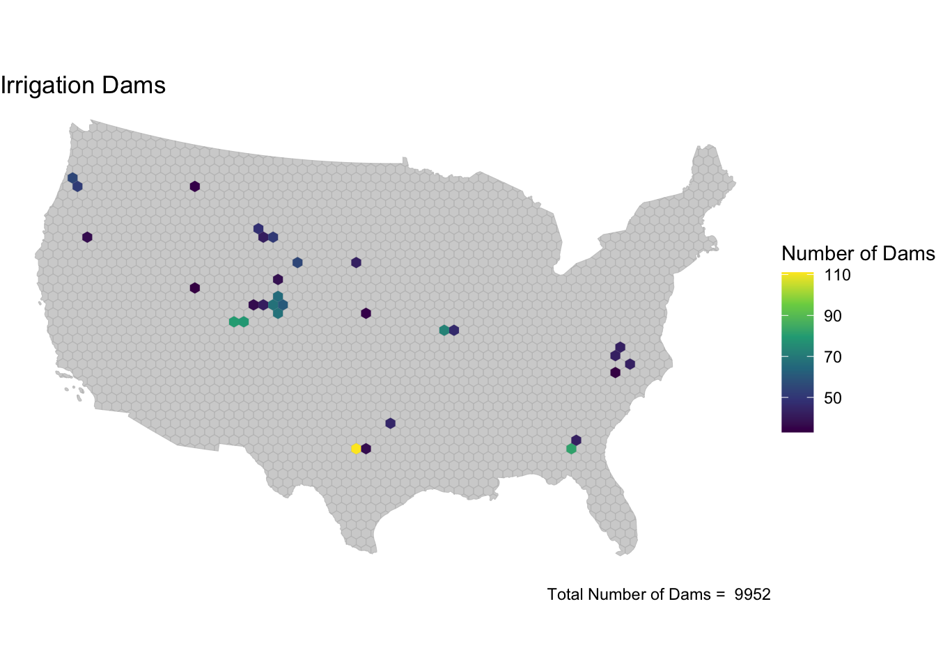
Water Supply Dams
dam_plot_funct(Hex_supply, "Water Supply Dams")+
  gghighlight(n > threshold)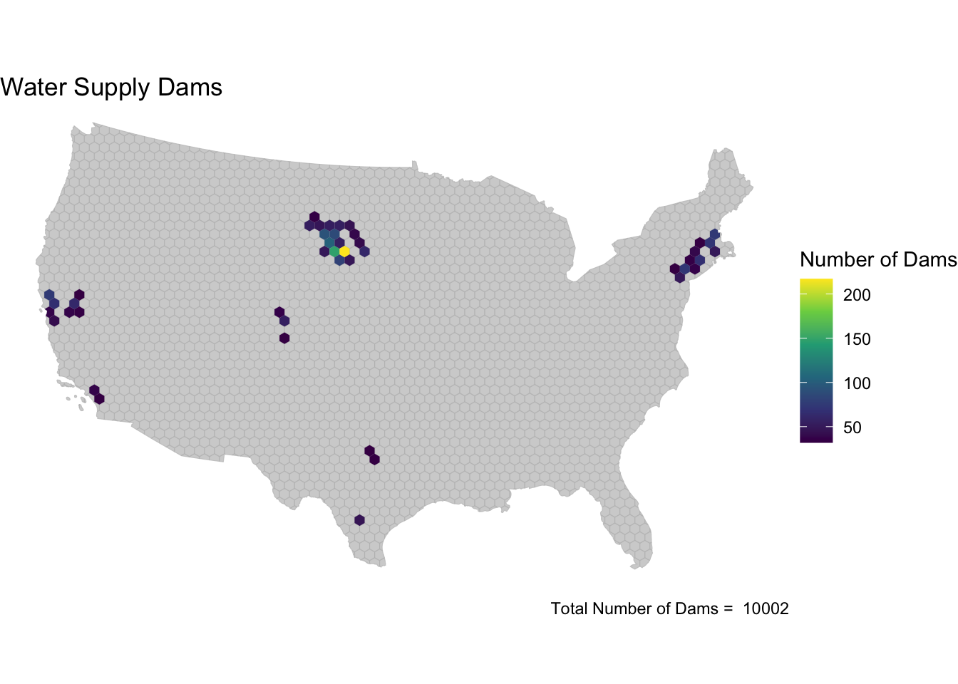
Fish and Wildlife Dams
dam_plot_funct(Hex_fish, "Fish and Wildlife Dams")+
  gghighlight(n > threshold)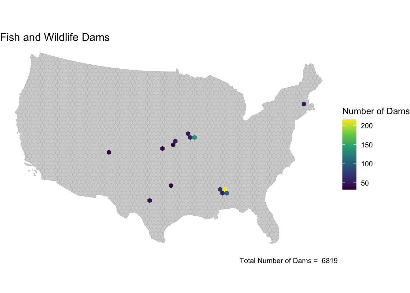
Step 4.3
After looking at the major purpose dams that i had picked i noted a couple of trends. Irrigation dams are located across the entire county. They seem to follow the middle of the county with a bit of a higher concentration in the rocky mountains. When looking at flood control dams these follow the wettest parts of the county. The Mississippi basin has some of the most water in the county and most of these dams are not massive but there are a lot to prevent flooding. Water supply dams make sense. There is a small concentration of them in New York but this is the biggest city in the world without a lot of freshwater availability. Also we can see that a lot fo dams are in the west and throughout the drier parts of the county. Finally as to my surprise all of the fish dams are concentrated in the Midwest to south. I had always imagined these dams would be priorities in the west.
Question 5
# read in major river data
major_rivers <- read_sf("majorrivers_0_0/MajorRivers.shp")

mississippi_river <- major_rivers %>%
  filter(SYSTEM == "Mississippi") %>%
  st_transform(crs = 4326)
# Filter for high risk flood dams
high_risk_dams <- dams %>%
filter(grepl("C", PURPOSES), HAZARD == "H") %>%
group_by(STATE) %>%
slice_max(NID_STORAGE, n = 1) %>%
ungroup() %>%
st_transform(crs = 4326)Build the Map
leaflet() %>%
  addProviderTiles(providers$CartoDB.Positron) %>%
  addPolylines(data = mississippi_river, color = "blue", weight = 2) %>%
  addCircleMarkers(
    data = high_risk_dams,
    radius = ~NID_STORAGE / 1500000,
    color = "red",
    fillOpacity = 0.8,
    stroke = FALSE,
    # Cannot get leafem to work
    popup = ~paste0(
      "<b>Name:</b> ", DAM_NAME, "<br>",
      "<b>Storage:</b> ", format(NID_STORAGE, big.mark = ","), "<br>",
  "<b>Purpose:</b> ", PURPOSES, "<br>",
  "<b>Year:</b> ", YEAR_COMPLETED
    )
  )